
Geometric Construction of Tangents to Richmond Curve
Loading the math board and drawing, please wait…
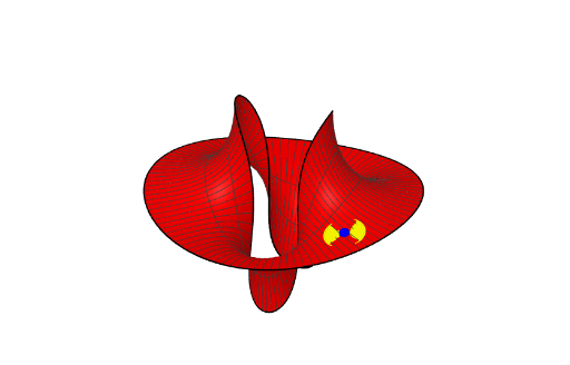
This GeoGebra example demonstrates the interactive construction of tangents to a specific curve known as the Richmond curve, illustrating the geometric relationship between curves and their tangents. Key mathematical concepts involved include tangents, derivatives, geometric construction techniques, and the local properties of curves within coordinate geometry. The construction utilizes commands such as Surface to create a surface context, CurveCartesian for plotting Cartesian curves, Sequence to generate point sequences, ClosestPoint for identifying nearest points, Tangent for tangent construction, and supporting commands like Line, OrthogonalLine, and Circle for auxiliary elements. Objects including parameters a, n, Rmax, Rmin, c, b, d, and others allow for dynamic adjustments of curve properties and tangent positions. This example is suitable for educational purposes in high school or university settings, particularly in analytic geometry and calculus courses, to provide an intuitive understanding of tangent concepts and their applications.
GeoGebra Commands & Parameters
Surface(((-cos(t))) / r - (r^((2 * n) + 1) / ((2 * n) + 1) * cos((((2 * n) + 1) * t))), ((-sin(t))) / r - (r^((2 * n) + 1) / ((2 * n) + 1) * sin((((2 * n) + 1) * t))), ((((-a)) / n * r^(n)) * cos((n * t))), r, Rmin, Rmax, t, 0, (2 * π)) → cCurveCartesian(((-cos(t))) / Rmax - (Rmax^((2 * n) + 1) / ((2 * n) + 1) * cos((((2 * n) + 1) * t))), ((-sin(t))) / Rmax - (Rmax^((2 * n) + 1) / ((2 * n) + 1) * sin((((2 * n) + 1) * t))), ((((-a)) / n * Rmax^(n)) * cos((n * t))), t, 0, (2 * π)) → bCurveCartesian(((-cos(t))) / Rmin - (Rmin^((2 * n) + 1) / ((2 * n) + 1) * cos((((2 * n) + 1) * t))), ((-sin(t))) / Rmin - (Rmin^((2 * n) + 1) / ((2 * n) + 1) * sin((((2 * n) + 1) * t))), ((((-a)) / n * Rmin^(n)) * cos((n * t))), t, 0, (2 * π)) → dSequence(Segment[b((i * π / 4)), d((i * π / 4))], i, 1, 7, 2) → liste1CurveCartesian(((-cos(tl))) / r - (r^((2 * n) + 1) / ((2 * n) + 1) * cos((((2 * n) + 1) * tl))), ((-sin(tl))) / r - (r^((2 * n) + 1) / ((2 * n) + 1) * sin((((2 * n) + 1) * tl))), ((((-a)) / n * r^(n)) * cos((n * tl))), r, Rmin, Rmax) → eClosestPoint(e, AL) → ALPTangent(ALP, e) → kCurveCartesian(((-cos(tl + dt))) / r - (r^((2 * n) + 1) / ((2 * n) + 1) * cos((((2 * n) + 1) * (tl + dt)))), ((-sin(tl + dt))) / r - (r^((2 * n) + 1) / ((2 * n) + 1) * sin((((2 * n) + 1) * (tl + dt)))), ((((-a)) / n * r^(n)) * cos((n * (tl + dt)))), r, Rmin, Rmax) → lClosestPoint(l, ALP) → ALPPCurveCartesian(((-cos(tl - dt))) / r - (r^((2 * n) + 1) / ((2 * n) + 1) * cos((((2 * n) + 1) * (tl - dt)))), ((-sin(tl - dt))) / r - (r^((2 * n) + 1) / ((2 * n) + 1) * sin((((2 * n) + 1) * (tl - dt)))), ((((-a)) / n * r^(n)) * cos((n * (tl - dt)))), r, Rmin, Rmax) → llClosestPoint(ll, ALP) → ALPQLine(ALPQ, ALPP) → mOrthogonalLine(ALP, Plane[k, m]) → pCircle(ALP, rayon, p) → q