
Generalized Logistic Differential Equation
Loading the math board and drawing, please wait…
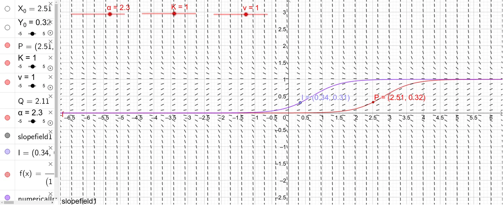
This example demonstrates the slope field and numerical solution of the generalized logistic differential equation, involving core concepts like differential equations, trigonometric functions, solids or 3D shapes, general quadrilaterals, power functions, and rhombuses. Using GeoGebra commands SlopeField and SolveODE, it visualizes the effects of parameters X_0, Y_0, P, K, ν, Q, α on the solution, suitable for high school and above students learning about applications and visualization of differential equations.
GeoGebra Commands & Parameters
SlopeField(((α * (1 - (y / K)^(ν))) * y), 200) → slopefield1SolveODE(((α * (1 - (y / K)^(ν))) * y), x(I), y(I), 10, 0.1) → numericalIntegral1SolveODE(((α * (1 - (y / K)^(ν))) * y), x(I), y(I), -10, 0.1) → numericalIntegral2
AI Drawing Prompt Reference
Create a slope field for the generalized logistic differential equation dy/dx = α(1-(y/K)^ν)y, using short line segments to show the direction at many grid points. From a given initial point, draw two smooth solution curves extending in positive and negative x-directions, following the slope field. The curves should illustrate how the solution evolves with parameters α, K, ν, and initial conditions. Ensure the slope field and curves are clearly visible, with the curves passing through the field to show the relationship between the differential equation and its numerical solutions.
The prompt above was compiled from the original drawing commands and is for reference only.