
Dispersion of White Light by Prism
Loading the math board and drawing, please wait…
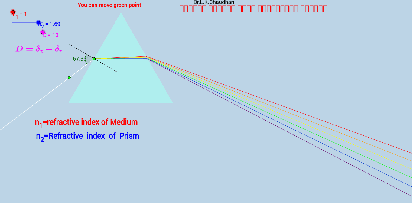
This example demonstrates how a prism disperses white light. Key mathematical concepts include refraction and dispersion. Using GeoGebra commands such as Point, Polygon, OrthogonalLine, etc., the path of light through the prism is constructed. Suitable for high school physics and mathematics education.
GeoGebra Commands & Parameters
Point(xAxis) → APolygon(A, B, 3) → poly1, c, a, b, CPoint(b) → D_2OrthogonalLine(D_2, b) → ePoint(e) → FPoint(e) → GAngle(F, D_2, E) → αRay(D_2, E) → dSlope(d) → mRotate(G, asin((n_1 / n_2 * sin(α))), D_2) → G'Ray(D_2, G') → fIntersect(a, f) → HSegment(H, D_2) → gOrthogonalLine(H, a) → hPoint(h) → IAngle(D_2, H, I) → γPoint(h) → JRotate(J, (-asin((n_2 / n_1 * sin(γ)))), H) → J'Angle(J', H, J) → δRay(H, J') → iSegment(F, G) → jSegment(J, I) → kAngle(G, D_2, G') → βRotate(G, asin((n_1 / (((1 + (0.002 * D)) * n_2)) * sin(α))), D_2) → PRotate(G, asin((n_1 / (((1 + (0.004 * D)) * n_2)) * sin(α))), D_2) → QRotate(G, asin((n_1 / (((1 + (0.006 * D)) * n_2)) * sin(α))), D_2) → RRotate(G, asin((n_1 / (((1 + (0.008 * D)) * n_2)) * sin(α))), D_2) → SRay(D_2, P) → sRay(D_2, Q) → tRay(D_2, R) → a_1Ray(D_2, S) → b_1Rotate(G, asin((n_1 / (((1 + (0.01 * D)) * n_2)) * sin(α))), D_2) → TRay(D_2, T) → c_1Intersect(a, s) → UIntersect(a, a_1) → VIntersect(a, t) → WIntersect(a, b_1) → ZIntersect(a, c_1) → A_1OrthogonalLine(U, a) → d_1OrthogonalLine(W, a) → e_1OrthogonalLine(V, a) → f_1OrthogonalLine(Z, a) → i_1OrthogonalLine(A_1, a) → l_1Point(d_1) → B_1Point(e_1) → C_1Point(f_1) → D_1Point(i_1) → E_1Point(l_1) → F_1Rotate(B_1, (-asin((((1 + (0.002 * D)) * n_2 / n_1) * sin(γ)))), U) → G_1Rotate(C_1, (-asin((((1 + (0.004 * D)) * n_2 / n_1) * sin(γ)))), W) → H_1Rotate(D_1, (-asin((((1 + (0.006 * D)) * n_2 / n_1) * sin(γ)))), V) → I_1Rotate(E_1, (-asin((((1 + (0.008 * D)) * n_2 / n_1) * sin(γ)))), Z) → J_1Rotate(F_1, (-asin((((1 + (0.01 * D)) * n_2 / n_1) * sin(γ)))), A_1) → K_1Ray(U, G_1) → nRay(W, H_1) → pRay(V, I_1) → qRay(Z, J_1) → rRay(A_1, K_1) → lSegment(D_2, U) → g_1Segment(D_2, V) → h_1Segment(D_2, Z) → j_1Segment(D_2, A_1) → k_1Segment(D_2, W) → m_1Intersect(b, a) → KIntersect(b, c) → LIntersect(a, c) → MPolygon(K, L, M) → poly2, m_2, k_2, l_2