
Cylindrical Spiral and Cosine Curve Relationship
Loading the math board and drawing, please wait…
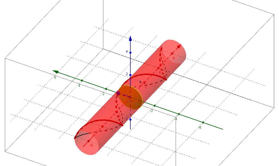
This example demonstrates the dynamic relationship between a cylindrical spiral and a cosine curve. It involves core mathematical concepts such as cylindrical spiral, cosine function, parametric equations, and analytical geometry. The construction utilizes GeoGebra commands like CurveCartesian for plotting curves, Segment for lines, Locus for creating paths, Circle for circles, and Surface for 3D surfaces. It is suitable for high school and above students to understand the connection between spatial curves and planar curves, as well as the application of parametric equations.
GeoGebra Commands & Parameters
CurveCartesian(t, cos(t), sin(t), t, -6.28319, 6.28319) → aCurveCartesian(t, cos(t), 0, t, -6.283185307179586, 6.283185307179586) → bSegment(C, A) → cSegment(B, C) → dLocus(B, θ) → loc1Circle(C, A, space) → eCircle(xAxis, A) → fSegment(B, A) → gSurface(u, cos(t), sin(t), u, -6.283185307179586, 6.283185307179586, t, 0, 6.283185307179586) → S
AI Drawing Prompt Reference
Draw a cylindrical spiral and a cosine curve to demonstrate their dynamic relationship. The spiral revolves around the z-axis while the cosine curve lies in the xy-plane. Connect key points with line segments, create paths and loci, and include two circles and a 3D surface to illustrate the connection between spatial and planar curves, emphasizing the use of parametric equations.
The prompt above was compiled from the original drawing commands and is for reference only.