
Cosine Function Demonstration by Richard Wade
Loading the math board and drawing, please wait…
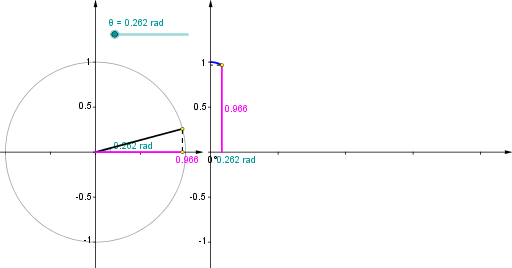
This example demonstrates the cosine function's graph and its geometric meaning, showing the calculation process through rotation and vector operations; core math concepts include cosine function, geometric transformations, vector operations, and parametric equations; construction highlights the use of GeoGebra commands/objects like Point, Rotate, Angle, Segment, Circle, Vector, Sequence, Function; suitable for high school mathematics teaching and function graph learning.
GeoGebra Commands & Parameters
Point(Ray[(0, 0), (-1, 0)]) → BRotate(A, θ, B) → PRotate(A, θ, B) → A'Angle(A, B, A') → αRotate(A, θ, B) → A'_1Angle(A, B, A'_1) → βSegment(Q, (x(Q), 0)) → eSegment((0, 0), (x(Q), 0)) → gCircle(B, A) → cSegment(B, P) → aVector((x(B), y(Corner[1])), (x(B), y(Corner[4]))) → uVector((0, y(Corner[1])), (0, y(Corner[4]))) → wVector((0, 0), (x(Corner[2]), 0)) → zSequence(Segment[((0.75 * i), 0), ((0.75 * i), -0.025)], i, 1, 4) → list1Segment(B, (x(P), 0)) → bSegment(P, (x(P), 0)) → hFunction(cos((120° * x)), 0, x(Q)) → fVector(B - (1.2, 0), B + (1.2, 0)) → vSequence(Segment[(0, (0.5 * i) - 1), (-0.025, (0.5 * i) - 1)], i, 0, 4) → list2Sequence(Segment[(x(B), (0.5 * i) - 1), (x(B) - 0.025, (0.5 * i) - 1)], i, 0, 4) → list3Sequence(Segment[B + ((0.5 * i) - 1, 0), B + ((0.5 * i) - 1, -0.025)], i, 0, 4) → list4Segment(Q, (0, y(Q))) → dPoint(Ray[(0, 0), (-1, 0)]) → B_1Rotate(A_1, θ, B_1) → P_1Rotate(A_1, θ, B_1) → A'_2Rotate(A_1, θ, B_1) → A'_3Circle(B_1, A_1) → c_1Segment(B_1, P_1) → a_1