
Concha (Euhoplites): Angle-driven optimization with circle/ellipse constraints
Loading the math board and drawing, please wait…
In collections
geometriadinamica.es
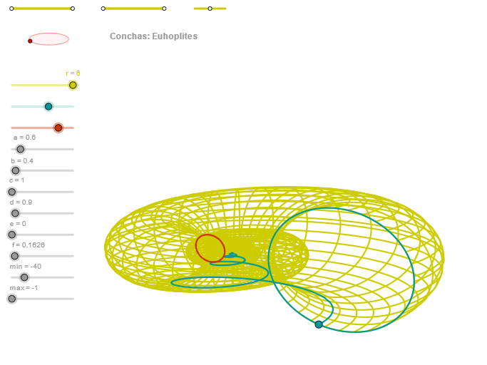
This example demonstrates how a geometry construction combining triangles, circles, and conic sections can visualize the behavior of a quantity under random/parameterized conditions, including its maximum and minimum values, along with the resulting curves or locus-like envelopes. Key concepts include analytic geometry (circle and ellipse construction), angle measurement (Angle), and optimization via max/min over parameter sets. From the GeoGebra construction summary, the build uses Segment and Point to set geometric anchors, OrthogonalLine to enforce perpendicular relationships, Circle plus Intersect to derive circle intersection constraints, Ellipse to create the conic boundary, Angle to define or control the critical angular measure, CurveCartesian to draw the corresponding Cartesian curve, and Sequence to generate parameter values for dynamic exploration. Suitable for high-school advanced learners and introductory university courses on geometry visualization, parameterized modeling, and optimization thinking.
GeoGebra Commands & Parameters
Segment(Q3, Q4) → p2Point(p2) → P3Segment(P3, Q4) → p4Point(p4) → P4Segment(Q1, Q2) → p1Point(p1) → P1Segment(P1, Q2) → p3Point(p3) → P2OrthogonalLine(C, yAxis) → zz1Circle(C, 0.62) → zz0Intersect(zz0, zz1, 1) → ZZ1Intersect(zz0, zz1, 2) → ZZ2Ellipse(ZZ1, ZZ2, 0.65) → zElipse1Intersect(zElipse1, zz1) → ZZ5, ZZ6Point(zElipse1) → XYAngle(ZZ6, C, XY) → zAngRotOrthogonalLine(C, xAxis) → zz2Intersect(zz0, zz2, 2) → ZZ3Intersect(zz0, zz2, 1) → ZZ4Ellipse(ZZ3, ZZ4, 0.65) → zElipse2Intersect(zElipse2, zz2) → ZZ7, ZZ8Point(zElipse2) → ZAngle(ZZ8, C, Z) → zAngIncSegment(Q5, Q6) → p5Point(p5) → P5Segment(ZZ5, ZZ6) → zz4Segment(ZZ7, ZZ8) → zz3Intersect(zElipse2, zElipse1, 1) → zPunto1Intersect(zElipse2, zElipse1, 4) → zPunto2Segment(zPunto1, zPunto2) → zSeg2CurveCartesian((r * ((((exp((f * u)) * (d + (a * cos(α)))) * cos((c * u))) * sin(zAngRot)) + (((exp((f * u)) * (d + (a * cos(α)))) * sin((c * u))) * cos(zAngRot)))), (r * ((((((-exp((f * u))) * (d + (a * cos(α)))) * cos((c * u))) * cos(zAngRot)) * sin(zAngInc)) + ((((exp((f * u)) * (d + (a * cos(α)))) * sin((c * u))) * sin(zAngRot)) * sin(zAngInc)) + ((exp((f * u)) * ((-1.4 * e) + (b * sin(α)))) * cos(zAngInc)))), u, u1, u2) → curva2CurveCartesian((r * ((((exp((f * β)) * (d + (a * cos(v)))) * cos((c * β))) * sin(zAngRot)) + (((exp((f * β)) * (d + (a * cos(v)))) * sin((c * β))) * cos(zAngRot)))), (r * ((((((-exp((f * β))) * (d + (a * cos(v)))) * cos((c * β))) * cos(zAngRot)) * sin(zAngInc)) + ((((exp((f * β)) * (d + (a * cos(v)))) * sin((c * β))) * sin(zAngRot)) * sin(zAngInc)) + ((exp((f * β)) * ((-1.4 * e) + (b * sin(v)))) * cos(zAngInc)))), v, v1, v2) → a1CurveCartesian((r * ((((exp((f * max)) * (d + (a * cos(v)))) * cos((c * max))) * sin(zAngRot)) + (((exp((f * max)) * (d + (a * cos(v)))) * sin((c * max))) * cos(zAngRot)))), (r * ((((((-exp((f * max))) * (d + (a * cos(v)))) * cos((c * max))) * cos(zAngRot)) * sin(zAngInc)) + ((((exp((f * max)) * (d + (a * cos(v)))) * sin((c * max))) * sin(zAngRot)) * sin(zAngInc)) + ((exp((f * max)) * ((-1.4 * e) + (b * sin(v)))) * cos(zAngInc)))), v, v1, v2) → curva1Sequence(CurveCartesian[(r * ((((exp((f * u)) * (d + (a * cos(v)))) * cos((c * u))) * sin(zAngRot)) + (((exp((f * u)) * (d + (a * cos(v)))) * sin((c * u))) * cos(zAngRot)))), (r * ((((((-exp((f * u))) * (d + (a * cos(v)))) * cos((c * u))) * cos(zAngRot)) * sin(zAngInc)) + ((((exp((f * u)) * (d + (a * cos(v)))) * sin((c * u))) * sin(zAngRot)) * sin(zAngInc)) + ((exp((f * u)) * ((-1.4 * e) + (b * sin(v)))) * cos(zAngInc)))), v, v1, v2], u, u1, u2, paso) → list2Sequence(CurveCartesian[(r * ((((exp((f * u)) * (d + (a * cos(v)))) * cos((c * u))) * sin(zAngRot)) + (((exp((f * u)) * (d + (a * cos(v)))) * sin((c * u))) * cos(zAngRot)))), (r * ((((((-exp((f * u))) * (d + (a * cos(v)))) * cos((c * u))) * cos(zAngRot)) * sin(zAngInc)) + ((((exp((f * u)) * (d + (a * cos(v)))) * sin((c * u))) * sin(zAngRot)) * sin(zAngInc)) + ((exp((f * u)) * ((-1.4 * e) + (b * sin(v)))) * cos(zAngInc)))), u, u1, u2], v, v1, v2, paso) → list1
AI Drawing Prompt Reference
Draw a geometric figure composed of triangles, circles, and ellipses, including two ellipses and one circle. Use the intersection points of the circle and ellipse to define key angles, and generate dynamic curves through angle and parameterized models to show the optimization process with maximum and minimum values.
The prompt above was compiled from the original drawing commands and is for reference only.