Complex Surface Demonstration

Loading the math board and drawing, please wait…

2015-10-26 07:37

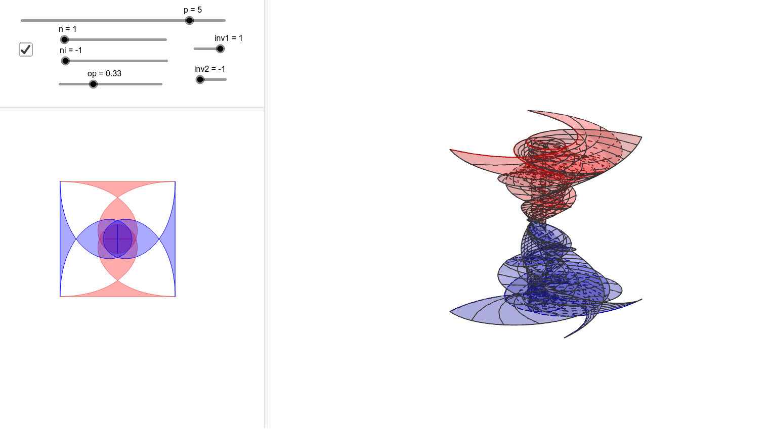
This example demonstrates the visualization and manipulation of complex numbers in three-dimensional space as surfaces. It involves core mathematical concepts such as complex numbers, surfaces, integral calculus, correlation, and difference/slope. The construction utilizes GeoGebra commands and objects like OrthogonalLine, Point, Sequence, and Surface as outlined in the summary. Suitable for high school and above, it aids in understanding the intersection of complex numbers and solid geometry.

GeoGebra Commands & Parameters

OrthogonalLine(a, yAxis) → c
Point(c) → A
Sequence(CurveCartesian[x((a + (r * t) + ((ί * r) * k))^(p)), y((a + (r * t) + ((ί * r) * k))^(p)), t, -1, 1], k, -1, 1, 1 / n) → liste5
Sequence(CurveCartesian[x((a - (r * k) + ((ί * r) * t))^(p)), y((a - (r * k) + ((ί * r) * t))^(p)), t, -1, 1], k, -1, 1, 1 / n) → liste6
Sequence(CurveCartesian[x((a + (r * t) + ((ί * r) * k))^(p)), y((a + (r * t) + ((ί * r) * k))^(p)), (p * inv1), t, -1, 1], k, -1, 1, 1 / n) → liste1
Sequence(CurveCartesian[x((a - (r * k) + ((ί * r) * t))^(p)), y((a - (r * k) + ((ί * r) * t))^(p)), (p * inv2), t, -1, 1], k, -1, 1, 1 / n) → liste2
Surface(x((a - (r * ni) + ((ί * r) * u))^(v)), y((a - (r * ni) + ((ί * r) * u))^(v)), (inv2 * v), u, -0.99, 1, v, 0.1, 6) → g
Surface(x((a + (r * u) + ((ί * r) * ni))^(v)), y((a + (r * u) + ((ί * r) * ni))^(v)), (inv1 * v), u, -1, 1, v, 0, 6) → b
Surface(x((a - (r * ni) + ((ί * r) * u))^(v)), y((a - (r * ni) + ((ί * r) * u))^(v)), (inv2 * v), u, -1, 1, v, 0, 6) → d
Surface(x((a + (r * u) + ((ί * r) * ni))^(v)), y((a + (r * u) + ((ί * r) * ni))^(v)), (inv1 * v), u, -1, 1, v, 0.1, 6) → f
Sequence(Surface[x((a + (r * u) + ((ί * r) * j))^(v)), y((a + (r * u) + ((ί * r) * j))^(v)), (inv1 * v), u, -1, 1, v, 0, p], j, -1, 1, 1 / n) → liste7
Sequence(Surface[x((a - (r * j) + ((ί * r) * u))^(v)), y((a - (r * j) + ((ί * r) * u))^(v)), (inv2 * v), u, -1, 1, v, 0, p], j, -1, 1, 1 / n) → liste8