
Binomial Distribution CDF (Static)
Loading the math board and drawing, please wait…
In collections
UNSW MATH1131/1231 Algebra material
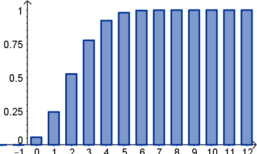
This example illustrates the cumulative distribution function (CDF) of the binomial distribution. It covers key concepts in probability and statistics. Using GeoGebra commands like Sequence and Join, it dynamically shows how the CDF changes with different parameters. Suitable for high school and above students or teachers to understand the probability accumulation process of the binomial distribution.
GeoGebra Commands & Parameters
Sequence(((n! / i! / (n - i)! * p^(i)) * q^(n - i)), i, 0, n) → fJoin({{0, 0, 0, 0, 0, 0, 0}, Sequence[Sum[Sequence[((n! / i! / (n - i)! * p^(i)) * q^(n - i)), i, 0, k]], k, 0, n], {1, 1, 1, 1, 1, 1, 1, 1, 1, 1, 1, 1, 1, 1, 1, 1, 1, 1, 1, 1, 1, 1, 1, 1, 1}}) → FSequence(Polygon[(i - d, 0), (i + d, 0), (i + d, Element[f, i + 1]), (i - d, Element[f, i + 1])], i, 0, n, 1) → PlotfSequence(Polygon[(i - 7 - d, 0), (i - 7 + d, 0), (i - 7 + d, Element[F, i + 1]), (i - 7 - d, Element[F, i + 1])], i, 0, n + 20, 1) → PlotF