
Basic Negative Power Functions
Loading the math board and drawing, please wait…
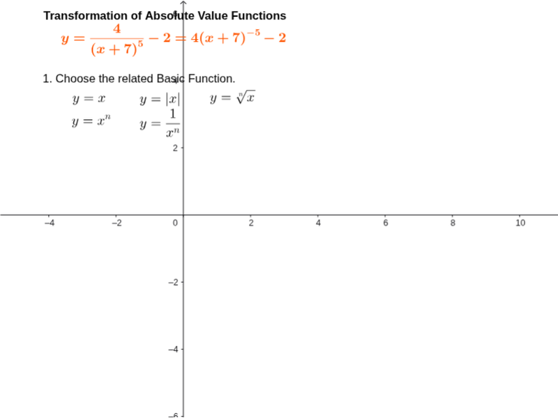
This example demonstrates the graph and properties of basic negative power functions. Key mathematical concepts include power functions, function transformations, and limits. Using GeoGebra commands such as Random, RandomElement, and If, users can dynamically adjust function parameters and observe changes in the graph. Suitable for high school mathematics education and learning.
GeoGebra Commands & Parameters
Random(-8, -1 + If[reset, 0, 0]) → nRandomElement(KeepIf[x ≠ 0, Sequence[i, i, ymin + 2, ymax - 2 + If[reset, 0, 0]]]) → aRandom(xmin + 1, xmax - 1 + If[reset, 0, 0]) → hRandom(ymin + abs(a), ymax - abs(a) + If[reset, 0, 0]) → vIf(Mod[n, 2] ≟ 0, 1, -1) → eo
AI Drawing Prompt Reference
Draw the graph of basic negative power functions to demonstrate function transformations and limits, with dynamically adjustable parameters to observe changes in the graph, including a randomly generated negative integer exponent, a non-zero real number coefficient, horizontal and vertical shifts, first determine the exponent and coefficient, then apply horizontal and vertical shifts, and finally plot the function graph to observe its changes.
The prompt above was compiled from the original drawing commands and is for reference only.