
Adding Fractions with an Area Model by Duane Habecker
Loading the math board and drawing, please wait…
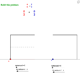
① This example demonstrates how to add fractions using an area model, turning abstract fraction arithmetic into a visual geometric representation. ② The core mathematical concepts include the meaning of fractions, addition of like and unlike denominators, and the geometric interpretation of common denominators (using least common multiples). ③ Construction highlights: using GeoGebra commands such as Point, Circle, Segment, Polygon, Sequence, GCD, and Mirror to build rectangular or square areas, generate dot arrays (DotsBottom, DotsTop) to represent numerators, compute common denominators via GCD, and partition regions with auxiliary lines and polygons (poly1, poly2, poly3) to show the combination of fractional parts. ④ Suitable for upper elementary to middle school students learning fraction operations, and useful for teachers in classroom demonstrations to foster intuitive understanding of fraction addition.
GeoGebra Commands & Parameters
Point(c) → ACircle(A, squaresize) → dOrthogonalLine(A, c) → eIntersect(d, e, 2) → B_1Intersect(d, c, 2) → CSegment(B_1, C) → fMirror(A, f) → A'Sequence((x(A) + (i * squareside / denominator2), y(A)), i, 1, denominator2) → DotsBottomSequence((x(B_1) + (i * squareside / denominator2), y(B_1)), i, 1, denominator2) → DotsTopPolygon(A, (x(A) + (numerator2 * squaresize / denominator2), y(A)), (x(B_1) + (numerator2 * squaresize / denominator2), y(B_1)), B_1) → poly1, a, h, i, jSequence(Segment[(x(A) + (i * squaresize / denominator2), y(A)), (x(B_1) + (i * squaresize / denominator2), y(B_1))], i, 1, denominator2) → DashedLines1Polygon(A, C, A', B_1) → poly2, a_1, c_1, a', b_1Point(c) → BCircle(B, squaresize) → gOrthogonalLine(B, c) → bIntersect(g, b, 2) → EIntersect(g, c, 2) → FOrthogonalLine(E, b) → kOrthogonalLine(F, c) → lIntersect(k, l) → GSequence((x(B), y(B) + (i * squaresize / denominator1)), i, 1, denominator1) → DotsLeftSequence((x(F), y(F) + (i * squaresize / denominator1)), i, 1, denominator1) → DotsRightSequence(Segment[(x(B), y(B) + (i * squaresize / denominator1)), (x(F), y(F) + (i * squaresize / denominator1))], i, 1, denominator1) → DashedLines2Polygon(B, F, (x(F), y(F) + (numerator1 * squaresize / denominator1)), (x(B), y(B) + (numerator1 * squaresize / denominator1))) → poly3, d_1, f_1, m, nPolygon(B, F, G, E) → poly4, d_2, f_2, g_1, e_1GCD(MixedNum, commondenom) → ReduceByRandom(2, 10) → seeddenominator1Random(2, 10) → seeddenominator2