
Roots of a Cubic Polynomial
Loading the math board and drawing, please wait…
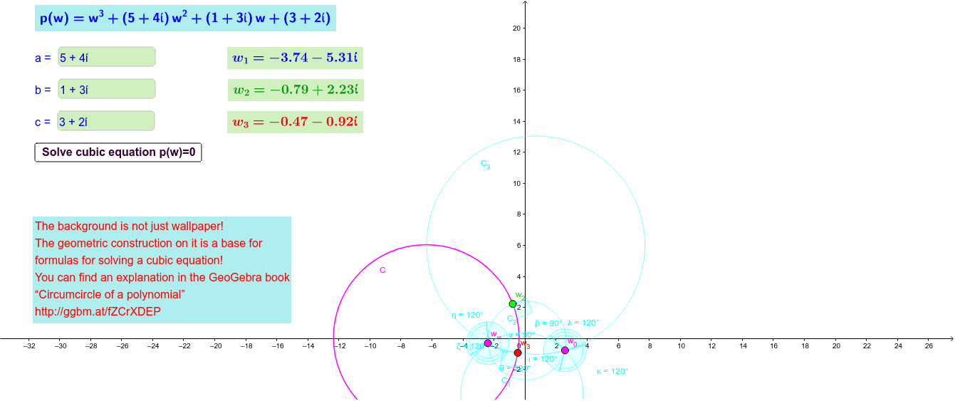
This example demonstrates the roots of a cubic polynomial. It involves the concept of polynomial functions and how to construct a cubic polynomial and its roots using GeoGebra commands. The construction summary mentions the use of Textfield, Circle, Point, Ray, Angle, Defined, etc. It is suitable for high school mathematics education or learning.
GeoGebra Commands & Parameters
Textfield(a) → InputBox1Textfield(b) → InputBox2Textfield(c) → InputBox3Text(w_1) → t1Text(w_2) → t2Text(w_3) → t3Circle(w_1, w_2, w_3) → CCircle(w_0, w_∞, w_1) → C_1Circle(w_0, w_∞, w_2) → C_2Circle(w_0, w_∞, w_3) → C_3Point(j_2) → B_2Point(j_3) → B_3Point(j_1) → B_1Ray(w_∞, B_2) → r_2Ray(w_∞, B_3) → r_3Ray(w_∞, B_1) → r_1Angle(r_3, r_2) → ζAngle(r_2, r_1) → ηAngle(r_1, r_3) → θPoint(h_1) → F_1Point(h_3) → F_3Point(h_2) → F_2Ray(w_0, F_1) → k_1Ray(w_0, F_3) → k_3Ray(w_0, F_2) → k_2Angle(k_1, k_2) → ιAngle(k_2, k_3) → κAngle(k_3, k_1) → λAngle(f_1, g_1) → αAngle(f_2, g_2) → βAngle(f_3, g_3) → γDefined(Center[C]) → qDefined(Center[C_1]) → q_1Defined(Center[C_2]) → q_2Defined(Center[C_3]) → q_3