
Plotting Parametric and Polar Curves
Loading the math board and drawing, please wait…
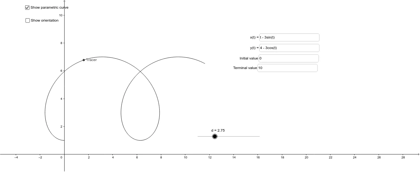
This example demonstrates how to plot parametric equations and polar curves using GeoGebra. It involves core math concepts like parametric equations, polar coordinates, function graphing, and trigonometry. Key GeoGebra commands and objects used include Segment, Sequence, Zip, Point, Textfield, Take, and Locus for dynamic visualization. Suitable for high school and above students to explore the applications of parametric and polar equations.
GeoGebra Commands & Parameters
Segment(O, A) → bSequence(Interval_{min} + (t * (Interval_{max} - Interval_{min}) / n), t, 1, n) → t_nZip((f(t), g(t)), t, t_n) → list1Point(b) → BTextfield(f) → inputBox1Textfield(g) → inputBox2Textfield(Interval_{min}) → inputBox3Textfield(Interval_{max}) → inputBox4Take(list1, 1, n - 1) → list2Take(list1, 2, n) → list3Zip(Vector[v_1, v_2], v_1, list2, v_2, list3) → list4Locus(Tracer, d) → loc1
AI Drawing Prompt Reference
Plot a parametric and polar curve. First, draw a line segment b between points O and A. Then, generate a sequence of t values based on the input minimum and maximum interval. Next, calculate the values of the parametric equations f(t) and g(t) for these t values to form a series of points. Connect these points to create the parametric curve. Finally, trace the movement of points to draw the polar curve.
The prompt above was compiled from the original drawing commands and is for reference only.