
Orthogonal Trajectories of Hyperbolas
Loading the math board and drawing, please wait…
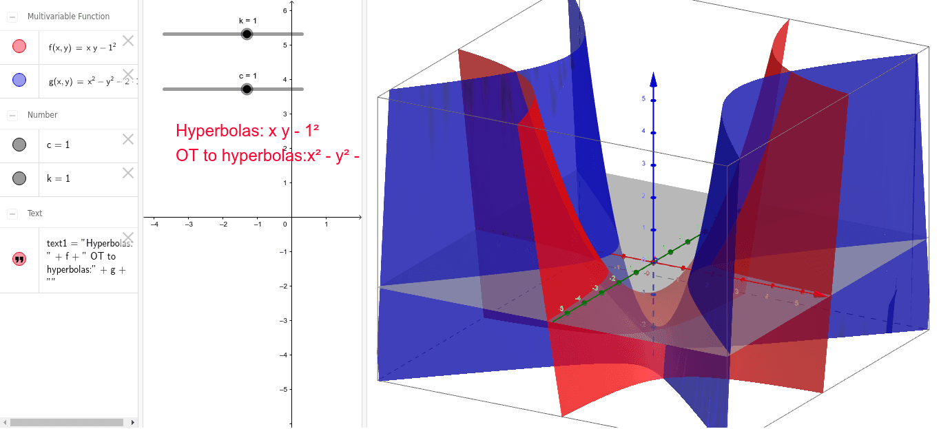
This example demonstrates the graphical relationship between a family of hyperbolas and their orthogonal trajectories. Key mathematical concepts include the trajectory equations in analytical geometry, orthogonality of curve families, and the application of parametric equations. Construction highlights involve using GeoGebra objects k (parameter), f (function), c (constant), g (graphics object), and text1 (text annotation) to dynamically visualize the variations in the hyperbola family and its orthogonal trajectories. Suitable for high school and above students to understand the geometric properties of curve families and the construction of orthogonal trajectories.
GeoGebra Commands & Parameters
Numeric k(1.0)f(x, y) = (x * y) - k^(2)Numeric c(1.0)g(x, y) = x^(2) - y^(2) - (2 * c)
AI Drawing Prompt Reference
Draw a family of hyperbolas and their orthogonal trajectories. First, plot the hyperbola xy=k^2 with k=1, then plot the hyperbola x^2-y^2-2c=0 with c=1, and observe their orthogonal relationship. By changing the values of k and c, dynamically show the variations in the family of hyperbolas and their orthogonal trajectories.
The prompt above was compiled from the original drawing commands and is for reference only.