
From Circular Motion to Graphs of Trigonometric Functions
Loading the math board and drawing, please wait…
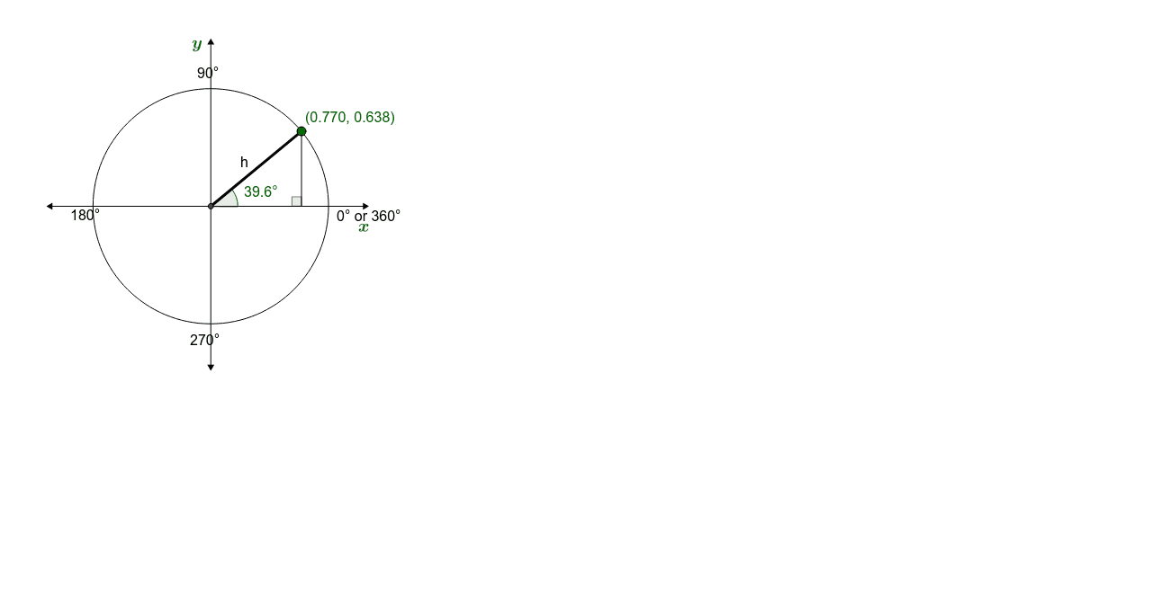
①This example dynamically demonstrates how sine, cosine, and tangent function graphs are generated from circular motion on the unit circle, linking geometric movement to function plots. ②Core mathematical concepts include definitions of trigonometric functions, the unit circle, angle-radian correspondence, and the periodicity, amplitude, and phase shifts of function graphs. ③Construction highlights: using GeoGebra commands such as Circle, Point, and Intersect to build the unit circle and moving point; OrthogonalLine, Segment, and Ray to draw perpendiculars and tangents; Angle and Function to mark angles and compute trigonometric values; and Point with Locus to trace the moving point's path, forming the function graphs. ④Suitable for high school trigonometry lessons, this serves as a classroom demonstration or self-guided exploration tool to help students understand the transition from geometric definitions to function graphs.
GeoGebra Commands & Parameters
Intersect(xAxis, yAxis) → AFunction(0, 1.9, 5.5) → gPoint(g) → QPoint(yAxis) → BCircle(A, B) → cPoint(c) → DTangent(D, c) → e,Intersect(e, yAxis) → FIntersect(xAxis, e) → ESegment(F, E) → lSegment(E, A) → mIntersect(m, l) → OIntersect(c, xAxis, 2) → CSegment(A, C) → dOrthogonalLine(D, d) → fIntersect(f, m) → HSegment(A, H) → cosαAngle(Q, A, D) → αSegment(A, D) → bSegment(D, E) → tanαSegment(D, H) → sinαOrthogonalLine(D, sinα) → iFunction(sin((2 * (x - (2 * 3.14 / 3)))), 2.09, 5.24) → sineαIntersect(sineα, h, (2.439250960476847, 0.6379515420040821)) → IFunction(tan((2 * (x - (2 * 3.14 / 3)))), 2.09, 5.24) → tangentαIntersect(tangentα, h, (2.439250960476847, 0.8284261815090247)) → JFunction(cos((2 * (x - (2 * 3.14 / 3)))), 2.09, 5.24) → cosineαIntersect(cosineα, h, (2.439250960476847, 0.770076509221398)) → KSegment(H, D) → jSegment(A, F) → kIntersect(j, m) → NIntersect(k, l) → PFunction(1, 1.9, 5.5) → pFunction(-1, 1.9, 5.5) → qPoint(c) → RSegment(C, R) → aSegment(A, H) → g_1Segment(D, H) → h_1Segment(A, E) → j_1Angle(A, D, E) → βRay(D, F) → i_1Ray(D, E) → l_1Intersect(c, a) → G, LOrthogonalLine(I, xAxis) → d_1Intersect(g, xAxis, 1) → MIntersect(g, xAxis, 1) → SIntersect(g, xAxis, 1) → TIntersect(g, d_1) → USegment(I, U) → e_1OrthogonalLine(K, xAxis) → k_1Intersect(k_1, xAxis) → VSegment(K, V) → m_1OrthogonalLine(J, xAxis) → n_1Intersect(n_1, xAxis) → WSegment(J, W) → p_1Point(yAxis) → ZPoint(yAxis) → A_1Segment(Z, A_1) → q_1Point(xAxis) → B_1Point(xAxis) → C_1Segment(B_1, C_1) → r_1OrthogonalLine(D, r_1) → c_1Intersect(g, r_1, 1) → D_1Intersect(c_1, r_1) → E_1Segment(D, E_1) → s_1Angle(D, E_1, A) → γ
AI Drawing Prompt Reference
Draw a unit circle and coordinate axes with the origin as the center. Place a moving point on the circle and draw a ray from the origin to the point. Drop perpendiculars from the moving point to the x-axis and y-axis, meeting them at points E and F respectively. Connect E and F, then draw a perpendicular from the origin to this line segment, meeting it at point O. Draw a tangent to the circle, meeting the x-axis at point C and the tangent at point D. From D, drop a perpendicular to the tangent, meeting it at point H. Draw line segments from the origin to D, H, and E, and label them sinα, cosα, and tanα respectively. Finally, plot the graphs of sinα, cosα, and tanα to show their relationship with the unit circle.
The prompt above was compiled from the original drawing commands and is for reference only.